Categories
Morse Code

Morse Sound to CW-Keyer Adapter Circuit

A transistor adapter circuit without need for external power supply converts Morse sound output to switch signals for the CW-keyer input of modern ham radio transceivers. In a simple variation, Morse sound signals directly drive the base of an all-purpose NPN transistor. Alternatively, a more robust design features a transformer and rectifier stage for improved switching signal accuracy and galvanic isolation.

The design idea of the two adapter circuits is to use the voltage on the transceiver’s keyer jack as a power supply.

Simple CW-Keyer Adapter

Simple sound card to CW-Keyer adapter.
Figure 1: Simple adapter from sound card output to CW-keyer signal.

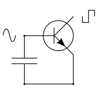
The most basic solution coming to mind has the sound card signal directly on the base of the switching NPN transistor. On the left hand side of Figure 1, the sound card of a laptop that generates the Morse code audio connects to the circuit. To the right it’s the keyer input of the transceiver.

In order to drive the base, Morse audio generators need to deliver signal levels above base voltage threshold. This should be no problem with computer sound cards. For instance, my laptop produces sound signals above 3.4 V peak to peak. As a switching transistor, BC 337 can be swapped with a wide variety of general-purpose NPN types.

On the Yaesu FT 991, Yaesu FT-DX 10, and Icom 7300 ham radio transceivers I tested, the keyer inputs correspond to voltage sources of +3 to +5 V with internal resistances of several kilo ohms. Consequently, the adapter has no need for an additional power supply and any NPN transistor can handle the low switching currents.

Simple adapter signals plot.
Figure 2: Simple adapter signals plot with incoming audio in yellow, collector voltage in green and transmitter RF output in blue.

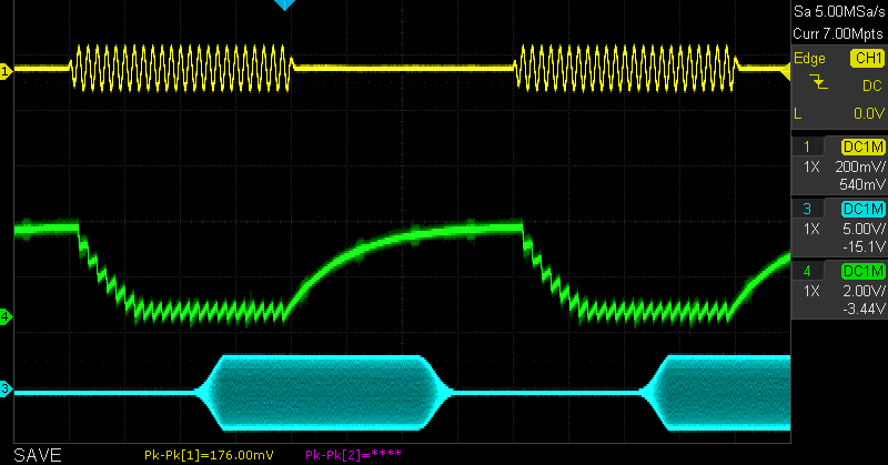
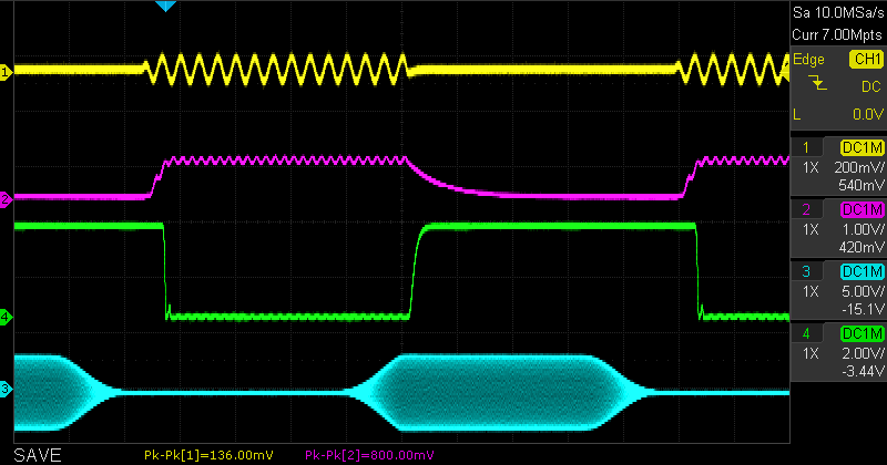
Figure 2 shows top yellow the Morse sound signal (in vertical scale 1:10), the keyer input / collector voltage green in the middle, and the transmitter output light blue on the bottom. Horizontally, one grid square is 10 milliseconds. In the adapter’s input path, the 4.7 kΩ and 4.7 nF constitute a low pass. On the output side the purpose of the 1 μF electrolyte capacitor is to cover the gaps between peaks of the sound signal.

Simple Morse Sound to CW-Keyer Adapter Board.
Figure 3: Simple Morse code to CW-keyer adapter board.

Downsides of the Simple Adapter Design

Because the transistor only conducts in its emitter-collector path when the base voltage crosses a threshold of roughly 0.6 V, a saw-tooth pattern is superimposed on the active sections of the green switch signal. At a side tone frequency of 600 Hz, gaps have lengths of about 1.5 ms. Therefore, the capacity on the collector side is not an easy choice. It needs to be big enough to sufficiently suppress the saw-tooth. But not be too big because otherwise the keyer voltage does not recover quickly enough during Morse code spaces.

The problems in finding a good value for the collector side capacitor is a fundamental weakness of the simple adapter. To make matters worse, the internal resistance of the keyer voltage source will differ between transceiver brands and models. So the 1 μF which I picked for my FT-DX 10 and speeds of up to 30 wpm may not be applicable to other use cases.

However, one could simply increase the frequency of the Morse sound signal up to 8 kHz. This would shorten the gaps and allow for much lower capacities to still suppress the saw-tooth.

Robust CW-Keyer Adapter Design with Transformer and Rectifier

The more robust version of the adapter avoids the problems of finding a good value for the collector capacitor. Because of a 1:10 to 1:20 transformer, the audio voltage becomes high enough for a rectifier bridge. Past the rectifier stage the audio frequency doubles and therefore the gaps in the base current of the switching transistor shorten. Thus, it is easier to balance short keyer voltage recovery times against suppressing the saw-tooth signal. What’s more, the load capacitor covering the gaps has moved from collector to the base side of the transistor. As a consequence, the resistance discharging the load capacitor no longer depends on the transceiver model. So, the values of 33 nF and 100 kΩ should suit most everyone.

Circuit for robust Morse sound adapter with transformer and rectifier bridge.
Figure 4: Circuit for robust Morse sound to adapter with transformer and rectifier bridge.

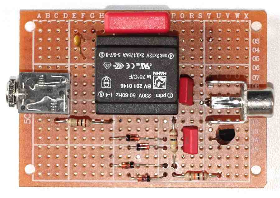
Since audio frequency transformers are getting rare, I just used a small sized power transformer. Translation ratios between 1:10 and 1:20, like 12V:230V, do the trick. Switching transistor and rectifier diodes can again be swapped for other general purpose types. If galvanic insulation is not important, one could replace the 470 nF capacitor with a wire bridge. Otherwise, a relatively large capacity needs to prevent interfering signals between the ground connectors from triggering the rectifier stage.

Robust adapter signals zoom view.
Figure 5: Robust adapter signals at 5 ms per grid square. Audio signal top yellow, rectifier output in purple, keyer voltage in green, and RF output light blue.

Signals for the more robust adapter converting Morse sound to CW-keyer input are shown in Figure 5. As expected, ripples on the purple driver voltage have double the sound frequency because of the rectifier.

Robust adapter signals at 50 ms per grid square.
Figure 6: Robust adapter signals for a 50 wpm Morse input at 50 ms per grid square horizontal resolution.

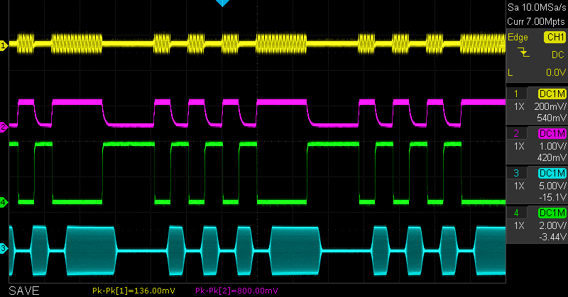
Overall, the robust adapter produces a clean switch signal with balanced dot and space ratio.

Robust Morse sound to CW-keyer adapter board.
Figure 7: Robust Morse sound to CW-keyer adapter implementation with transformer and rectifier.

Conclusion

Electronic adapter circuits to turn computer generated Morse code audio into transceiver suitable switch signals are easy to implement. Without need for external power supply, as well as optional galvanic input and output separation, the design minimizes the risk of short-circuit faults, which is great for portable operation. And for self-written Morse code software, audio streams are a good choice to achieve millisecond precision signal timing.

Categories
Testimonials

Antennas Amplifiers 4m 4El Yagi PA70-4-1.5B

Antennas Amplifiers’ 4 element yagi for the 4m / 70MHz ham radio band makes a good overall impression. It took me less than two hours to assemble and mount it on my telescoping tower. Soon after, I had my first amateur radio connections on 70 MHz in the log.

Antennas Amplifiers PA70-4-1.5B 4 element 4m yagi.
Figure 1: Antennas Amplifiers PA70-4-1.5B 4 element yagi for 4m ham radio band on my telescoping tower.

Shipping and Packaging

Ordered from WiMO[2], the antenna shipped in four business days. Packaging is 1.49 m long, just so it fits the 1.47 m boom. Element rods came grouped by size in cling wrap. All hands-on in sympathetic small business look and feel.

Packaging of the antenna.
Figure 2: packaging of the antenna with parts in cling wrap.

Initially I was interested in the 3 element version because I was concerned that the 4 element might be too hard to handle on my balcony. Since it was sold out in Germany, I even considered ordering it directly from Goran YU1CF[1]. However, shipping from Serbia is said to be slow and costs 40€. In the end, I decided to do a bit heavier lifting and went for the 4 element variant.

Assembly

The enclosed English manual does not cover the PA70 types specifically. It just contains some technical details for a variety of antenna products. For me this wasn’t an issue as all parts are clearly labeled, making the assembly fairly self-explanatory.

Mounting elements to the boom.
Figure 3: Assembly detail mounting elements to the boom.

Antenna elements numbered 1 – 4 with letters A and B indicating sides are all matched by labels sticking to the aluminum boom.

Antenna element assembly.
Figure 4: Antenna element assembly with labels and drill holes for self-tapping screws.

Furthermore, labels E1 through E8 mark where smaller and larger diameter pipes that make up the elements fit together. Push in the smaller pipes until both drill holes for self-tapping screws overlap. Afterwards put in the screws to secure the elements. One little point of critique: I might have wished for slightly smaller drill holes to give the screws a better grip.

Fixing balun to active elements.
Figure 5: Fixing the balun to the active elements of the antenna.

My next complaint is that I could not find a wrench to tighten the screws that fix the balun connectors to the active elements. Even with some more space around the screws the cable roll still blocks the access. This was the only part of the assembly that I found a bit fiddly.

Operating the Antennas Amplifiers PA70

The 4 element yagi is very lightweight and easy to lift onto a telescoping tower. Due to the relatively thin elements its wind load is low and in my setup it has an SWR of less than 1.2 on 70.154 MHz without tuning. I lack the equipment to measure radiation patterns, but when targeting stations, the antenna’s directivity meets my expectations for a 4-element beam.

In all, the PA70-4-1.5B makes a good first impression and is lightweight enough for balcony operation. The antenna’s boom is 1.47 meters and the reflector element 2.17 meters long.

References

[1] 4 meter 4 element Portable Antenna PA70-4-1.5B 70MHz, Antennas Amplifiers / Dual

[2] YU1CF PA70 Yagi, WiMO

Categories
Verticals

Multi-Band with 5.6m Fishing Rod Vertical Dipole

Setup for a ham radio vertical dipole of 5.6 meter fishing rod length that works multi-band 40 to 10 meters with inductive loading. No need for radials because of K9YC style ferrite chokes. Design suits restricted space balcony or portable operation.

As a regular K9YC vertical, the system covers the 17 to 10 meter bands using a transceiver-side antenna tuner. However, the proposed asymmetric loading technique achieves far superior performance on the 17 and 15 meter bands. It moreover enables operation on the 20, 30 and 40 meter bands within the 5.6 meter size limit. Just by placing load coils off-center the design results in good SWR matches below 1.5.

Due to its lightweight construction, all it takes to support the vertical antenna is a telescoping fishing rod. An additional telescoping tower made of aluminum or steel lifts up the heavier ferrite chokes and lower end of the dipole.

I recommend reading this post on the purpose and construction of the ferrite RF chokes as an introduction.

SWR Matching of Vertical Dipoles Shortened by Inductive Load

It is well known to the ham radio community that shortening wire antennas by inductive loading reduces the feed impedance. For instance, the ARRL Antenna Book[1] has impedance tables for top and base loading of verticals, according to which the center feed impedance of a dipole shortened by factor four drops to below 5 Ω. To counteract this effect, moving away from the center increases the resistance of the feed point. Therefore, a combination of shortening by inductive loading and shifting the feed point adjusts the feed resistance to a wide range of target values, such as the 50 Ω commonly in use by ham radio transceivers.

For a better understanding of asymmetric designs I recommend checking out off-center-fed dipoles[2] like the Windom[3] antenna.

Because of the design of vertical dipoles with high impedance ferrite chokes, matching antennas by off-center feeds is especially unproblematic. Unlike the Windom[3] antenna, asymmetric vertical dipoles do not produce a heavy load of shield currents.

Shortened Vertical Dipole Wiring Scheme

Wiring scheme of shortened vertical dipole with dimensions.
Figure 1: wiring scheme for shortened dipole with RF choke and antenna sections.

Figure 1 shows the wiring scheme for the shortened dipole with RF choke, feeds and inductive load. Labels L1 through L4 identify the antenna sections for which dimensions are given in the next section. As explained in my post on K9YC Verticals, the RF choke serves to electrically separate the dipole from its feed.

Vertical Dipole Antenna Wires with Loads and Dimensions

Coil sections of vertical dipole antennas for multi-band operation.
Figure 2: coil sections of vertical dipole antennas for 40, 30, 20 and 15 meter amateur bands.

Figure 2 depicts load coils for 40, 30, 20 and 15 meter ham radio bands. All coils are fixed on the same kind of tubing for electrical installations available at hardware stores. The tubes are 2.54 cm (1 inch) in diameter and the enameled copper wires have thicknesses of 1.5 and 1.2 mm. Coils for 40, 30, 20, and 15 meters have 97, 55, 25, and 9 turns, respectively. In addition to the coils, the image also shows the RG 58 feed lines with just the inner conductor connecting to the L2 wire sections.

Since all the L1 feed sections are about the same length, it’s surprising that the L2 sections don’t vary much either. This is very likely not optimal and when I find the time, I may experiment some more.

Nevertheless, despite the similar wire lengths, in all of the configurations the feed point moves away from the center electrically. This is due to the growing portion of the full-sized dipoles that the inductive loads replace. As a result, the center point of the dipoles moves inside the inductive loads. This effect, in turn, electrically pushes the feed point towards the lower side of the antenna. So as the center impedance decreases with larger coils, the cancellation effect of the off-center feed point increases. At least, that’s my theory.

Having verified that my full-size vertical dipoles worked well, I actually expected to need impedance transformers on top of the load coils. But as is, the system performs much better on lower bands than I had hoped for. All the same, I think it might be worthwhile to optimize my dipoles with some modeling software.

Wire Lengths

BandL1L2L3L4
10/11m2.37n/an/a2.41
12m2.725n/an/a2.74
15m2.600.210.0352.505
20m2.610.190.072.47
30m2.630.170.1252.42
40m2.620.190.162.365
Table 1: Wire and coil lengths with labels as in Figure 1. All in meters.

Table 1 has the wire lengths for my configurations for 10 to 40 meters. The L1 numbers include the 12 cm from SO 259 plug of the wires to the first ferrite choke. Between 26.985 and 28.074 MHz I get an SWR of 1.6 or below. For 12 meters I used a low loss feed cable so I can match the wire between 18 and 30 MHz with an antenna tuner. However, on 21 MHz tuning losses are already quite significant. Setups with load coils for 15 to 40 meters are likely not optimized, but way better than the alternative of using a match-box. As mentioned before, it might still pay off to verify dimensions in a modeling software.

A rolled-up wire setup.
Figure 3: the setup for 15 meters rolled up.

Mounting and Changing Dipole Wires

One obvious downside of the verticals is the need to swap wires in order to change bands. But with some practice, the process is now relatively swift for me.

A simple knack to get wire on and then the coil over the rod is to first pass the end of the wire through the coil like in Figure 4. Then slide the coil over the black tip of the rod on the left hand side to get the end of the wire on the right hand side of the coil. Afterwards, with the rod pointing up vertically, push up the rod starting with the thinnest innermost segment. In the process it’s advisable to rotate segments to get the wire wrapped around the rod.

Pass the top end of the dipole back through the coil to fix it at the end of the fishing rod.
Figure 4: Pass the top end of the dipole back through the coil to fix it at the end of the fishing rod.

Also note the paper clip that I keep attached to the top of the rod with the white cord. It’s very convenient because the little ring that secures the wire quickly slides over. Keeping the clip tied at all times has the huge added benefit of not having to go fishing for the tip of the rod. Hold up the rod vertically and try to get out its smallest segment to see what I mean.

Tip of the rod with paper clip attached.
Figure 5: Tip of the outer segment of the rod with paper clip attached and rubber cap holding the cord in place.

When flipping wires I always keep the fishing rod’s rubber cap at hand. Not only does it protect the outer segment from damage, it’s also perfect to firmly hold the paper clip when attaching wires.

Tower and Rod in Operation

Collapsed telescoping tower with multi-band RF choke and extended fishing rod with load coil.
Figure 6: collapsed telescoping tower with multi-band RF choke and extended fishing rod.

Finally, my telescoping tower on the left and extended rod on the right side of Figure 6. I step on a ladder to clip in wires with RF choke and rod mounted on the collapsed tower. Note how the coil for the 40 meter band, pointed to by the orange arrow, hardly adds to the wind load of the rod. Similar for the ferrite chokes with a much smaller wind surface than an equivalent T2LT coil for 40 meters.

References

[1] Vertical Antennas, ARRL Antenna Book, 24th edition, Chapter 9.2

[2] Off-center-fed Dipoles, Hamradiosecrets.com

[3] Windom Antenna, W8JI

Categories
Verticals

Broadband RF Choke for K9YC Verticals

K9YC style verticals separate center-fed vertical dipoles from their coax feed lines by means of high impedance RF chokes. First, a short summary of Jim Brown’s original idea[3] and its mention in the ARRL Antenna Book[5]. I then describe my experiments in developing the high impedance broadband RF chokes that make this type of antenna possible.

The K9YC Vertical Dipole

The two halves of K9YC vertical dipoles consist of the shield of a coaxial feed line, and a wire connected to its inner conductor. At first glance they look like ground plane verticals without radials. But that’s because K9YC verticals are dipoles that don’t need radials as counterbalances.

Vertical dipole made of coax shield and the inner conductor extended with copper wire.
Figure 1: a K9YC vertical dipole made up by shield and extended inner conductor of a coaxial feed line.

Figure 1 has an idealized K9YC vertical dipole with feeding point in the center, as indicated by the two λ/4 halves and amplitudes of RF currents dashed in red. This configuration is equivalent to a perfect center-fed half-wavelength dipole. But unfortunately, it cannot be connected directly to coaxial feed lines without altering antenna characteristics. Effectively, a coax feed bringing a signal to the lower end of the dipole will turn the configuration into a quarter-wavelength vertical lacking radials.

K9YC’s solution to keeping the structure electrically isolated as well as connected to the transmitter line is to place an RF choke at its lower end. Figure 2 shows a schematic of the choke, which allows signals to pass from the feed line while blocking RF currents from the shield.

Wiring schema of K9YC  vertical dipole with RF choke blocking RF currents at the lower end.
Figure 2: wiring diagram having an RF choke at the bottom of the lower end of the vertical dipole.

Note that the K9YC design is quite similar to the T2LT. Instead of ferrite chokes the T2LT uses coil of coax feed line as a choke. To me the 8 to 12 cm diameter coils look like their impedance might well be boosted by resonance. If someone tried this, please fill in the gap as a comment.

In my experiments K9YC verticals work well with inductive loading for lower short wave bands.

Advantages of K9YC Vertical Dipoles with RF Choke

Before diving into details of constructing high-impedance RF chokes, some words on why radio hams might find the proposed vertical dipole useful. After all, the construction looks weird and is likely to be met with a good deal of skepticism. Some say it couldn’t possibly work at all due to a lack of radials. Others give it the benefit of doubt, but state that a regular ground-plane would still perform better. I feel such criticism is missing the whole point of using K9YC verticals.

First, vertical dipoles, including many popular CB antennas, are great solution for installations without room for radials. Second, ground-plane antennas only perform well with several radials at right angles. However, most ham ground planes work with only one radial per band. Third, K9YC verticals shift the feeding point half an antenna length up, thus gaining all-important height.

Broadband High Impedance RF Choke Design

Amidon FT-240 43 broadband ferrite toroid choke coiled with Sucoform 50 Ω microwave cable.
Figure 3: Amidon FT-240 43 ferrite toroid coiled with Sucoform 50 Ω microwave cable.

Broadband high impedance RF chokes can be implemented by winding coaxial cable through a ferrite toroid. Such chokes make use of the shielding effect of coaxial cables to separate signals from unwanted shield currents. For signals, the magnetic fields of the shield and the inner conductor cancel each other outwardly. Therefore, the ferrite choke will not attenuate signals between transceiver and antenna. In contrast, shield currents are not canceled out and therefore induce magnetic flux in the ferrite. This fact is well known to the ham community building cable trap baluns.

In summary, RF currents from the lower end of the dipole will “see” the coil as a resistance. However, the signals between transceiver and antenna are only subject to normal cable attenuation along the length of the cable wound through the ferrite.

Appropriate Choice of K9YC Broadband RF Choke Ferrite Material

Creating broadband high impedance RF chokes, I experimented with Amidon FT-240 43[1] and FT-240 77[2] ferrite toroids.

Amidon FT-240 43 with regular copper wire for impedance measurement.
Figure 4: Amidon FT-240 43 with regular copper wire for impedance measurement.

For the FT-240 43 the AL value from datasheet[1] is 1075 nH/turn, note my factor 106 conversion milli to nano. With 10 turns like in Figure 4 the trap coil should have an inductance of 107.5 μH.

L = 10^2 * 1075 * 10^-9 H
L = 1075 * 10^-7 H = 107.5 μH

Thus, at 7 MHz, the ferrite trap from Figure 4 has a theoretical reactance of XL = 4.7 kΩ. At 28 MHz, the reactance would be as high as 18.9 kΩ. See Appendix 1 giving some theoretical background.

XL = 2 * π * 7 * 10^6 * 107.5 * 10^-6
XL = 4728 Ω

In my installations, I aim for a reactance of at least 10 kΩ over the frequency range of 7 to 28 MHz. Then, theoretically, two FT-240 43 trap coils of ten turns each should suffice for K9YC verticals. Believing the datasheets, traps with FT-240 77 should work even better. Given their AL of 2590 nH/turn, at 7 MHz a 10 turn coil has a reactance of 11.4 kΩ. So one might think that a single coil should safely cover the entire frequency range.

However, measuring the actual resistances of coils, as shown in Figure 4, gives different results. I found that FT-240 77 is good for frequencies below 7 MHz at best. Vertical dipoles with RF chokes using FT-240 43 have much sharper resonances and perform noticeably better.

Practical Choke Implementations for Telescope Towers

Broadband RF choke with fishing rod, plastic tube and aluminum telescope tower.
Figure 5: FT-240 43 chokes in serial connection mounted to fishing rod, plastic tube and aluminum telescope tower.

Figure 5 shows my approach to mounting the K9YC RF choke on an aluminum telescope mast. The fishing rod serves to pull up the vertical dipole halves. A plastic pipe for electrical installations holds three series-connected inductor coils in a straight row. Installation clamps connect the rod, plastic tube and aluminum pipe.

For the Amidon FT-240 43 material I found no reasonable upper limit of turns using thin Sucoform[4] cable. I could fit 17 turns and estimated no decrease of impedance due to capacities or resonances on 28 MHz. I should mention that I am lacking dedicated equipment for measuring RF impedance. Presently, I am using a dedicated measurement circuit and a digital oscilloscope for this purpose.

Using expensive Sucoform microwave cable is probably overkill. Reduced capacitance and small bending radius aside the stiffness of this cable produces chokes of better mechanical stability.

Packaging and rain proofing of K9YC RF chokes.
Figure 6: packaging, rain proofing and mounting detail for the FT-240 43 RF chokes.

To protect them from the rain, I wrapped the ferrite cores in a freezer bag with the bottom open.

Mounting detail for tower to tube and fishing rod connection.
Figure 7: mounting detail for tower to tube and fishing rod connection with SO 259 socket.

I use installation clamps, available at most hardware stores, to attach the tower to the pole and also to attach the SO 259 sockets.

FT-240 77 variant of RF chokes using RG58 cable.
Figure 8: FT-240 77 variant of RF choke using regular RG 58 cable.

Figure 8 shows my other experiment building the K9YC from a serial connection of four FT 240-77 coils. This trap will be good for 160 m and medium wave antennas. While the Amidon 77 material is not well suited for frequencies above 3.5 MHz, the RG58 cable seemed to do the trick. I achieved highest impedance fitting 15 turns of RG58.

Trap distancing detail.
Figure 9: electrical installation tubes slightly larger in diameter ensures equal distancing of choke coils.

Finally, Figure 9 shows how plastic tubes from hardware stores with slightly larger diameters equally distance the four choke coils. This implementation is a bit over-designed for the kW power range. My other chokes are tested for up to 100 W output power.T

Short Anecdote how I came to use K9YC Verticals

I stumbled upon Jim Brown’s design reading the ARRL book after a stay at my parents’ house, following a sked with an old friend from CB times. As a 12 year old kid, my electronics and radio hobby started with partly home-made CB radios not too compliant with the strict German regulations of the time. Our equipment produced maybe 4 W of RF power, which was well above the 500 mW that Bundespost set as a legal limit for the legendary 12 channels AM. Looking back, it seems surprising such crappy transceivers allowed for stable connections in our small-town. Especially since my friend and I had trouble hearing each other on 21 MHz with modern ham-radio transceivers, ground-plane antennas and 100 W PEP in SSB.

So the much ridiculed CB technology must have done something right! And my only explanation is that our CB vertical antennas must have performed far superior to our amateur radio ground planes. In fact, the reason for the poor ham performance is painfully obvious. Multi-band ham radio verticals typically skimp on a single radial per band, turning the verticals into V-shaped dipoles with irregular radiation patterns.

For CB, we used either end-fed half-wave vertical dipoles, or 5/8 λ verticals. And while my “City Star” half-wave dipole performed slightly worse than 5/8 λ, it had the huge advantage of not requiring space for radials. Exactly the problem I still have as a big city apartment dweller!

Appendix 1: Computing Trap Coil Reactances

Calculating the expected inductance of ferrite toroid trap coils is straightforward. Simply multiply the AL value from datasheets with the square of cable turns!

L = AL * n2

L: coil inductance (in Henry)
AL: ferrite specific inductance per turn
n: number of turns

The impedance, or roughly resistance to shield currents, is now given by the well known formula for the reactance:

XL = ωL = 2 * π * f * L

XL: reactance (~ resistance)
π: ~ 3.141
f: frequency in Hz
L: inductance in H

References

[1] Amidon FT-240 43 Ferrite Toroid Data-Sheet

[2] Amidon FT-240 77 Ferrite Toroid Data-Sheet

[3] End Feeding a Center-Fed Vertical Dipole, Jim Brown K9YC

[4] Sucoform 86 FEP Low Loss Coaxial Cable

[5] Vertical Antennas, ARRL Antenna Book, 24th edition, Chapter 9.2